
PUMPCALC is a Centrifugal Pump Analysis program. It can be used to predict the performance of one or more centrifugal pumps, at various impeller sizes, speeds and series or parallel configurations.
|
The main features of PUMPCALC are: • Single pump performance - Impeller size and speed changes. • Multiple Pump Performance - Series and Parallel Configurations. • Viscosity Corrected Pump Performance - Hydraulic Institute method. • Pump Head Curve versus Pipe System Head Curve - Operating point. • Screen and printer graphic plots. |
|
The following is a brief summary of input data for and functionality of PUMPCALC:
The main data needed for running PUMPCALC is the pump performance data. This consists of sets of values of Flow rate (or capacity), Head and Efficiency for a particular pump, for a specific impeller size and speed.
Normally, you will need to get this information from a pump catalog. The number of sets of Flow, Head and Efficiency values are limited to between 3 sets of points (minimum) and 15 sets of points (maximum). The data points taken off of a manufacturer's pump curve must cover the entire range of flow rate permissible for the specific pump.
Extrapolation can be made but may result in inaccurate results. Pump data files are saved under a name with a PMP file extension, such as "Compton.PMP".
To create a new pump file, choose File from the main menu followed by New and enter data in the blank spreadsheet displayed below.
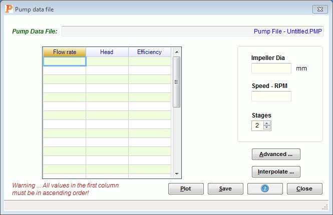
In addition to the three columns of data for Flow rate, Head and Efficiency, you may also specify the pump impeller size, speed and the number of stages in this pump. After entering all data, choose File/Save from the menu bar and save the pump curve data in a file name of your choice.
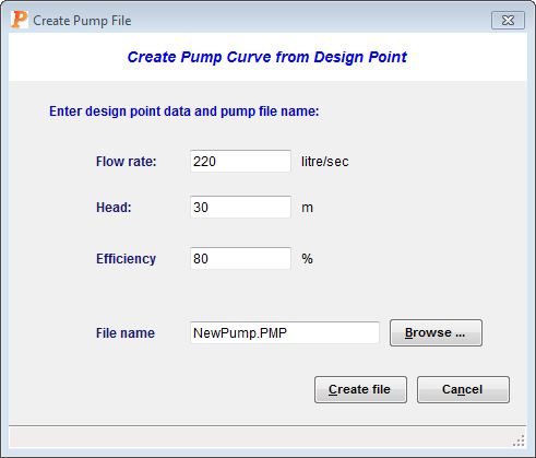
The Advanced... button above is for entering a single design point data for a pump, in order to create a typical pump curve. For example, if the desired design point is at 220 litre/sec, 30 m head at 80% efficiency, you may enter this data for PUMPCALC to automatically create a pump curve based on this design point, as shown in screen below.
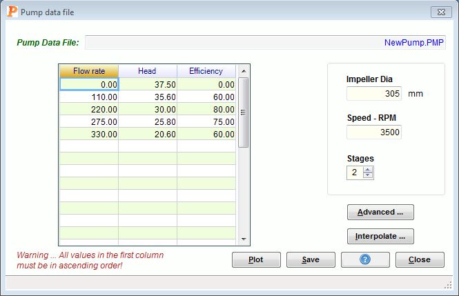
After entering data for the design point as above, and selecting a name for the pump file, click the Create file button. PUMPCALC will automatically create a pump curve for the design point specified as shown below. It can be seen that the pump curve data has been created around the best efficiency point (BEP) specified above.
The Interpolate... button is used to interpolate data from a given pump curve. Upon clicking this button the following screen is displayed:
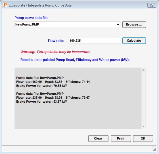
From this screen, you may interpolate the pump curve data for different flow rates. For example, at a flowrate of 160 l/s, the interpolated head and efficiency are 33.65 m and 74.4 % respectively. The brake power for water is also calculated and displayed as indicated above.
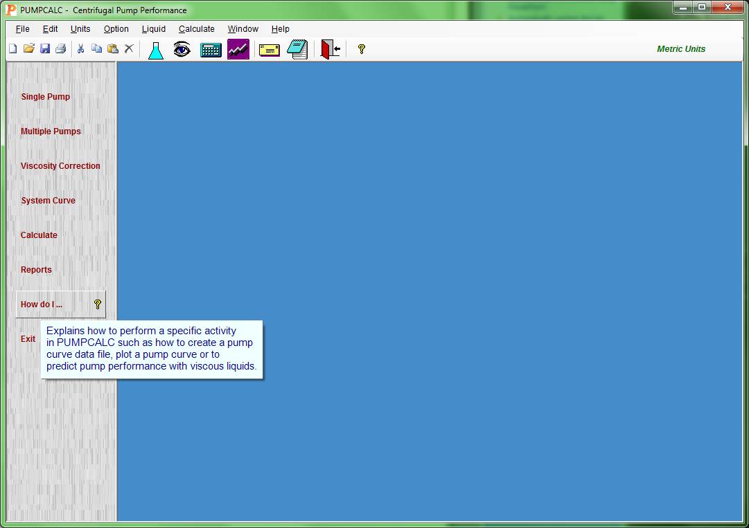
There are four main features of PUMPCALC, as indicated by the four buttons arranged vertically down on the left hand side of the main screen, shown below.
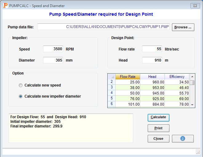
The button titled Single Pump is for calculating the performance of a single pump, determining its performance at different impeller diameters and speeds and generating a graphic plot of the Head, Efficiency and Power versus Capacity curves. Also, for a given Design Point (Q-H value), it can be used to calculate the new impeller size or speed.
The second button titled Multiple Pumps is for calculating the combined performance of two or more pumps in a series or parallel configuration.
The third button titled Viscosity Correction is for predicting the performance of a pump that pumps viscous liquids. For high viscosity liquids, the given water performance curve is used in conjunction with the built-in Hydraulic Institute charts to estimate the viscosity corrected pump performance. The resultant performance curves may be plotted on the screen as well the printer.
The fourth button titled System Curve is for calculating the System Head curve together with the pump curve when the pipe system characteristics are given. The point of intersection between the pipe system head curve and the pump curve can be determined using this option. For a given pipeline diameter, length and elevations, the system head curves can be generated for different liquid properties and the point of intersection of the pump curve and the pipeline system curve can be determined. Graphics of the combined pump performance versus the system curve are also generated.
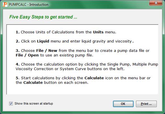
The list of the Five Easy Steps to get started with PUMPCALC is displayed when the program is launched, as shown below:
Choosing the Single Pump option displays the following:
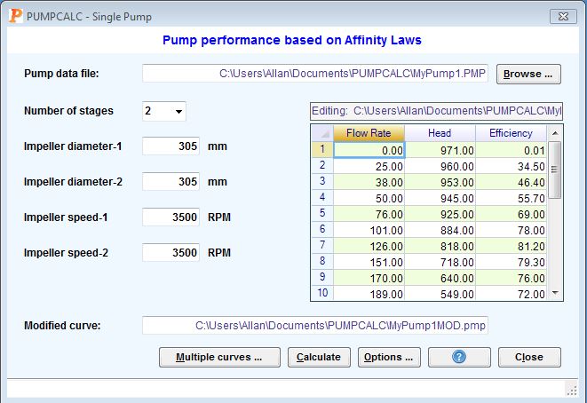
Using Affinity Laws, the pump performance at different impeller diameters and speeds can be calculated, from the given pump curve data based on a particular impeller size and speed. Also, for a specific design point (head and capacity values), the program can predict the impeller size or pump speed required, based on the existing impeller size and speed.
Clicking the Options... button in the above screen displays the following for specifying the required design point (Q-H values):
Clicking the Multiple curves... button displays the following for inputting the diameters or speeds required for generating a family of Head-Capacity curves, based on Affinity Laws:
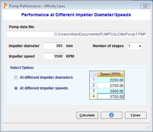
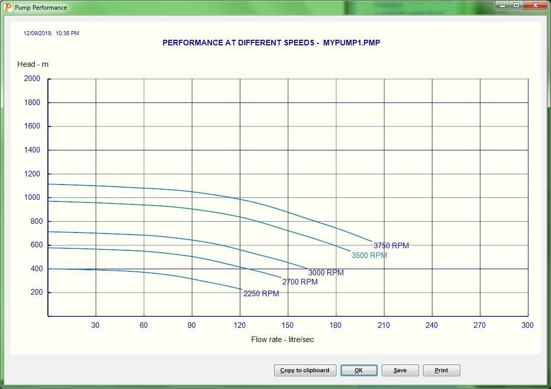
A family of pump Head versus Capacity curves may be generated from given pump data at various impeller sizes or pump speeds, using the Affinity Laws. The results of the above are shown in the following plot:
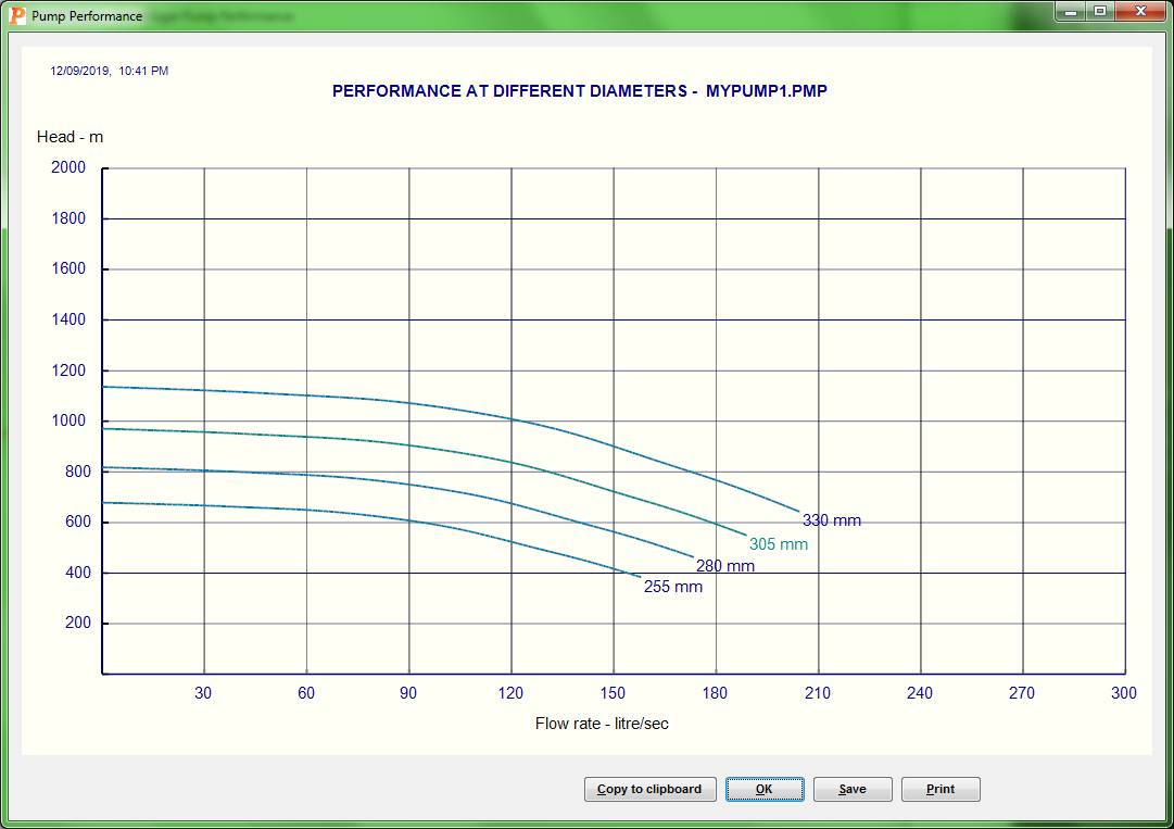
If the impeller diameter variation option were chosen, instead of speed variation, the following family of H-Q curves will be generated:
Clicking the Multiple Pumps button from the main screen displays the following for entering pump data to calculate the combined pump performance in a Series or Parallel configuration:
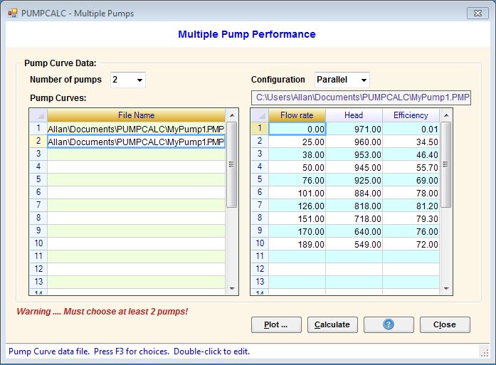
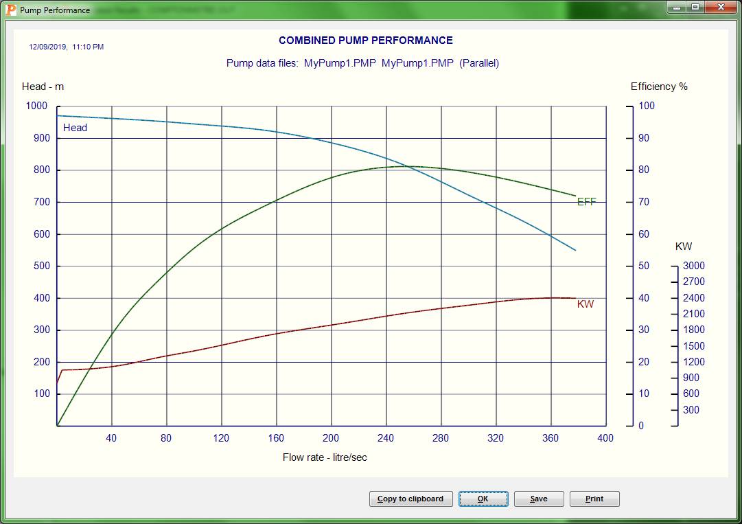
After entering the data for pumps, clicking the Calculate button will display the calculated results for the combined pump performance. The screen graphics of the combined pump performance will also be displayed, based on the plot option chosen from the following screen:
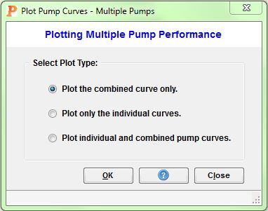
The combined pump performance may be plotted as follows:
Clicking the Viscosity Correct button displays the following for inputting the pump and liquid data for performing the viscosity correction, using the Hydraulics Institute chart method:
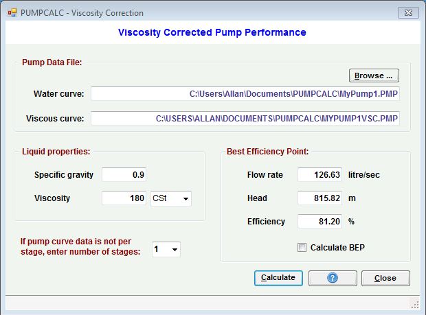
Enter the file name of the water performance curve and the file name for storing the viscosity corrected performance data. Press F3 to view a directory listing of available pump data files to choose from. Only those pump files with a PMP extension will be displayed. The file name for the viscous curve, by default, has the letters VSC added to the pump file name. For example, if the water curve is Pump1.PMP then the viscous curve will be shown as Pump1VSC.PMP.
The viscous performance calculated requires the use of the Best Efficiency Point (BEP) from the water curve. This is defined as the point on the water performance curve with the maximum efficiency. The flow rate, head and efficiency at this point on the curve is used as the starting point for viscosity corrected performance calculations. The BEP values may be specified in the appropriate fields or you may have PUMPCALC calculate the BEP by interpolation. After entering all data, click on the Calculate button to start calculations. Based on the Hydraulic Institute Charts, the water performance curve will be corrected for the given liquid viscosity. The water performance curve and viscous performance curve calculated will shown side by side in spreadsheets as shown below:
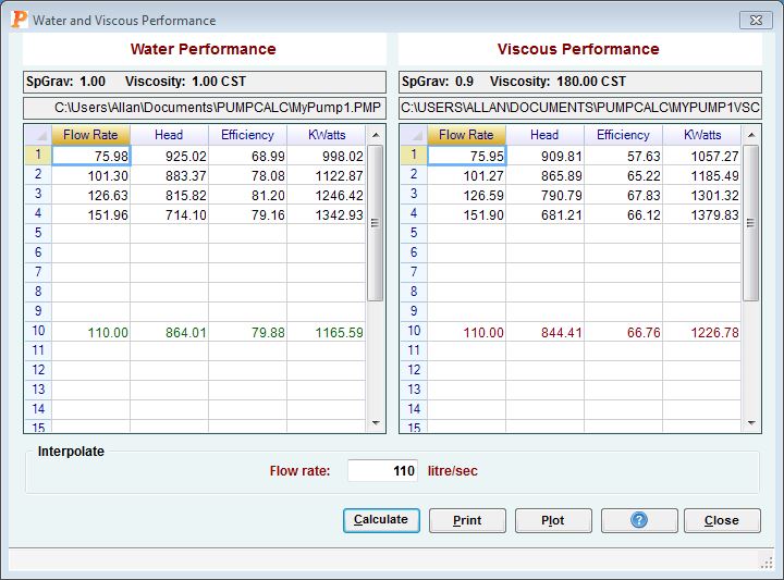
It must be noted that the results displayed are for only the four sets of data (60% BEP, 80% BEP, 100% BEP and 120% BEP) for both water curves as well as the viscous curves, in accordance with the Hydraulic Institute method.
Once the viscous performance is calculated, additional points on the viscous curve can be determined by interpolation. If the water performance and the corresponding viscous performance are desired at a particular flow rate, enter this value in the Flow rate field as shown above and click the Calculate button. The performance on both curves at the specified flow rate will be calculated and displayed on the spreadsheets, in a highlighted color. Similarly, additional data points on both curves can be calculated.
Remember that extrapolating beyond the limits of the performance curve, though feasible, may be inaccurate. Due to the nature of the Spline Interpolation method used, extrapolation may, in some cases yield incorrect results. However interpolation is generally quite accurate. The calculated viscous performance curve is saved in a data file as shown in screen above. This curve information may subsequently be used with the Single Pump option to determine other performance characteristics using the affinity laws.
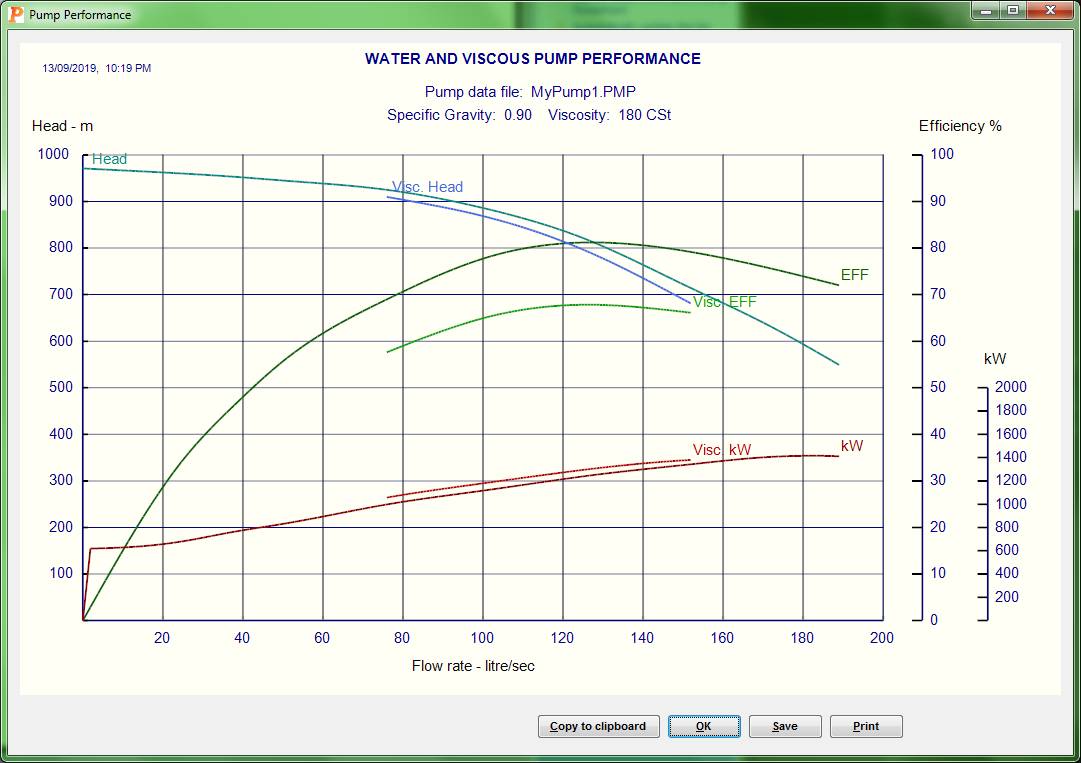
Clicking the Plot button on the viscosity correction screen above opens another windows to choose the type of plot. The calculated water performance and viscous performance curves can be plotted by clicking one of the option buttons.
Clicking the System Curve button on the main PUMPCALC screen displays the following window for inputting the pump and pipe data for calculating the System Head curve and operating point. The latter is the point of intersection between the system head curve and the combined pump performance curve. The liquid properties data input screen should also be checked to ensure that the correct liquid data (specific gravity and viscosity) is used in these calculations.
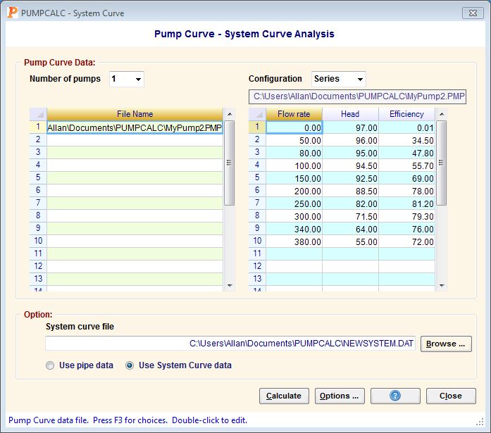
Clicking the Options... button in the above screen displays the window for inputting the additional pipe data needed for generating the system head curve similar to the following:
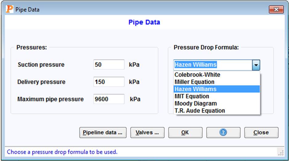
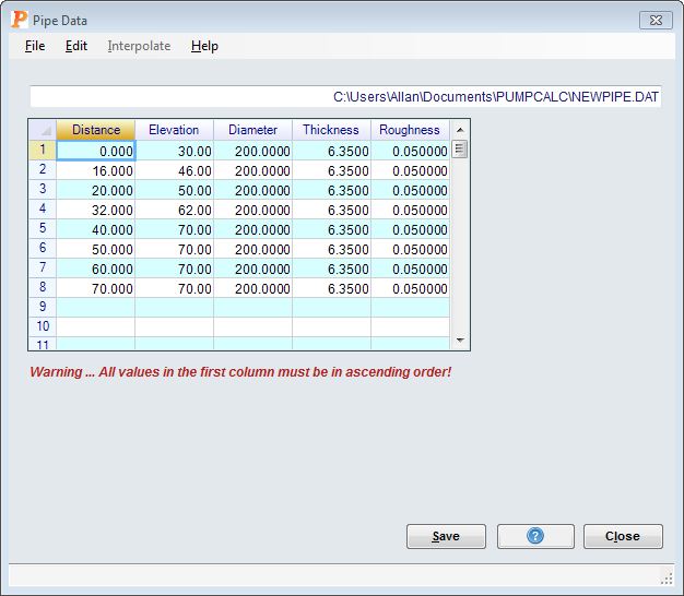
For calculating the pipe system head curves, the pipeline data (distance, elevation, diameter, wall thickness and pipe roughness) are input and stored as a data file. The liquid specific gravity and viscosity are input under the separate Liquid screen, from the menu on the main PUMPCALC screen. The pump suction pressure, pipe delivery pressure, maximum allowable pipe pressure and the pressure drop formula are also input in the screen above.
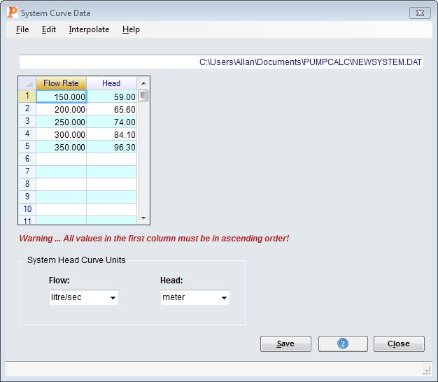
Alternatively, instead of pipe data above, the system head curve may be directly input. This option allows you to enter the Flow rate versus System head data for plotting against the pump head curve. If the System Head curve data is input, PUMPCALC ignores the pipe data and uses the system head curve data, without calculating the pressure drops.
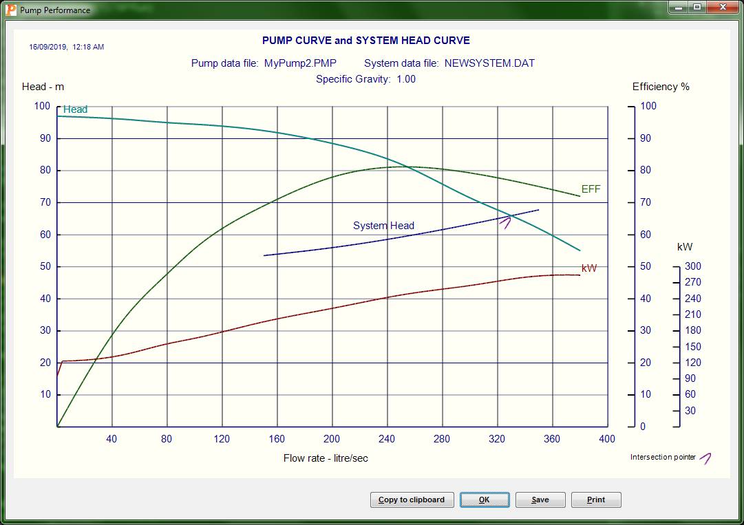
When used with the given pipeline data, in the absence of system head curve information, pipeline pressures are calculated for various flow rates to generate the System Head curve. Hydraulic calculations are performed based on the chosen pressure drop formula, such as Colebrook-White, Moody, Hazen-Williams, MIT or Miller equation for isothermal conditions of flow. The output consists of the pump operating flow rate, discharge pressure, efficiency and power at the operating point. Charts of the combined pump curve and system head curve are also generated as shown below:
Extrapolation of curve data:
Although PUMPCALC provides an option for the extrapolation of pump curve data beyond the values input by user, this can some times result in inaccurate results. Use this option with caution!
Always try to include sufficient points (up to a maximum of 15 sets) from the manufacturer's pump curve data covering the full range of flow rates anticipated. Do not depend on PUMPCALC to extrapolate performance data beyond the range of values input.
Similarly, if using the System Head curve input option, provide enough data for the system head curve covering the full range of flow rates anticipated, including the maximum pump flow rates permissible for the pump curves selected.
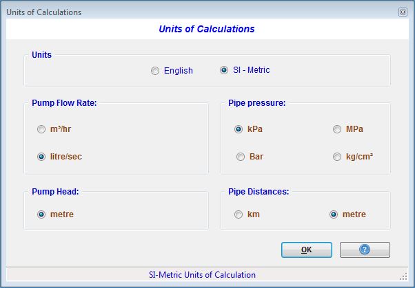
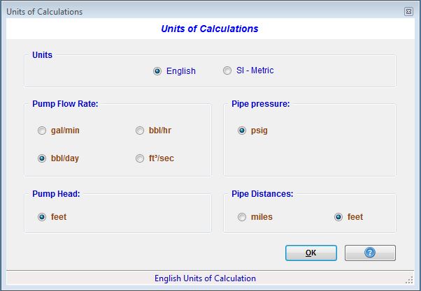
English and Metric units for calculation are available.
|
|
Refer also to SYSTEK (www.systekus.com/downloads/PUMPCALC.htm)
Computer Requirements
This program runs on a Windows 32 bit platform such as Microsoft Windows® 7 to 11, Vista and Microsoft Windows® XP SP3.